
What is linear Regression?
Wikipedia states – In statistics, linear regression is a linear approach to modeling the relationship between dependent variable and one or more independent variables.
Linear regression is a basic and commonly used type of predictive analysis.
Back to school math, every straight line can be represented by the equation: y = mx + b, where y is dependent variable and X is the independent variable on which y depends.
How can we use regression for a real life use case?! Let’s take an example – what if I have data of past 5-10 years on the quantity of wheat produced annually. With Linear regression, I will be able to predict what the wheat production would be this year or a year from now.
Why is prediction so important? It helps us plan and be prepared. It helps us deal with unforeseen situations. In the context of above example, a country will know the quantity of wheat it can export/import in a year. It means, if global demand seems much lower than the quantity we foresee producing, we can help farmers choose some other crop, since less demand means a bare minimum selling rate.
Some additional use cases:
- A consistent increase in Blood pressure and sugar levels, Is the patient heading towards heart attack?
- A distinctive seismic activity, are we in for a tsunami /earth quake?
- Inward migration of birds increasing on yearly basis. Are a certain species of trees responsible for alluring birds?
- Will a certain steel stock move up or down this year?
These are all some basic uses cases of Linear regression model. We call it regression, because we will be predicting continuous values (as opposed to a yes or no result). Graphically, a linear equation (with one dependent and one independent variable) looks similar to this
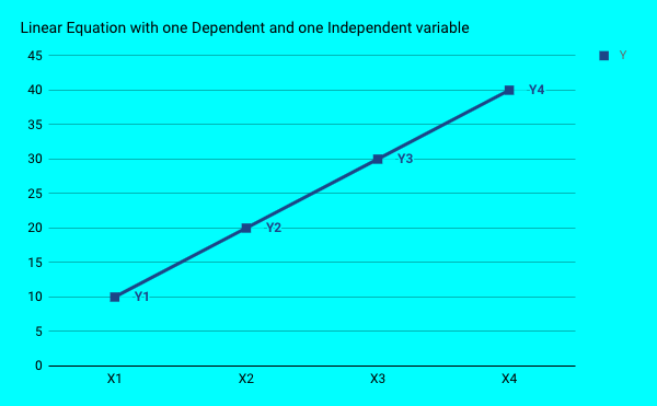
So, for every X , we can derive the value of Y from the equation.
What happens if Y is dependent on , not just one independent variable (X) but few more variables. The graph above will have not just X,Y axis but Z axis too to represent the second independent variable. More than two independent variables are hard to depict graphically. But, can be represented quite easily with equation as
y= β + β1×1 + β2×2….
where β 1,β2…βn are coefficients of X1, X2,X3
β is the y-intercept
What this implies for our wheat production example is:
y(total wheat produced in a year) = β + β1*Total available land in acres + β2 * rainfall received for that year + β3 * fertiliser availability in the market….. Here, rainfall received, fertiliser availability are the added independent variables apart from the size of land in acres.
Where does Machine Learning come into picture?
In the above equation – β1, β2, β3…are all coefficients whose value we need to compute to form the linear equation. This is where learning happens. Based on past data, ML learns the values of these coefficients through a number of iterations.
How?
To start with, we feed in data of past few years to ML packages, this is called training data, since it helps train the ML model. Through a large chunk of data and a number of iterations, the model learns the values of each of the coefficients.
We can then evaluate the model, ML packages offers a lot of functions and related parameters to know how the model has performed. Based on these values we decide if the model has learnt “enough” and then use this on the data we need to predict for (test data).
What is the error people talk about in ML?
If all data points (Y1,Y2,Y3….) form a perfect linear line as shown above, we can derive an exact output (prediction) we are looking. But, in the real world, this is not the case. The data points do not exactly form a line. They are a bit scattered on the graph. So what do we do? We make a line in such a way that its at a least possible distance from the points as shown below:
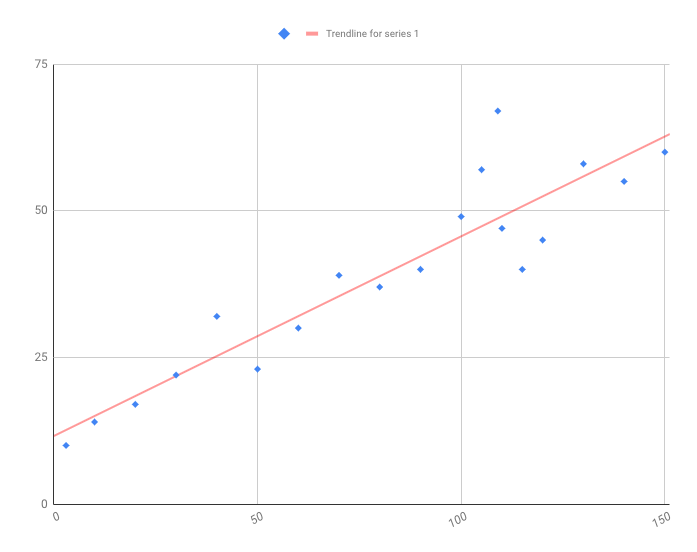
this is where root mean square error or any other error reduction method is used. So, we use the chosen method, and come out with a line (which best depicts the given data points)as output. Based on this line we predict the outcome, this is where our final values come from.
Let’s look at a very basic example of linear regression in PySpark
I have downloaded the dataset from https://www.kaggle.com/leonbora/analytics-vidhya-loan-prediction
- creating a Spark session
from pyspark.sql import SparkSession

spark = SparkSession.builder.appName('lr_example').getOrCreate()
2. Importing Linear Regression packages
from pyspark.ml.regression import LinearRegression
3. We will read the input data and see its structure
data = spark.read.csv("train.csv",inferSchema=True,header=True)
data.printSchema()
#output looks similar to this
root
 |-- Loan_ID: string (nullable = true)
 |-- Gender: string (nullable = true)
 |-- Married: string (nullable = true)
 |-- Dependents: string (nullable = true)
 |-- Education: string (nullable = true)
 |-- Self_Employed: string (nullable = true)
 |-- ApplicantIncome: integer (nullable = true)
 |-- CoapplicantIncome: double (nullable = true)
 |-- LoanAmount: integer (nullable = true)
 |-- Loan_Amount_Term: integer (nullable = true)
 |-- Credit_History: integer (nullable = true)
 |-- Property_Area: string (nullable = true)
 |-- Loan_Status: string (nullable = true)
Machine Learning packages expect only numerical inputs and cannot accept strings. A lot of packages are present to help us transform our data to suit ML requirements. This, we will look at this aspect in another post. As of now, we will just consider two numerical fields from above data schema( ‘ApplicantIncome, CoapplicantIncome’) and we will try to predict ‘LoanAmount’ with these inputs.
4. All our input data needs to be in the form of Vectors, an input to ML packages. So, lets get this sorted first:
from pyspark.ml.feature import (VectorAssembler, VectorIndexer)
#lets define what inputs will go into our vector and give a name for the output of it
lassembler = VectorAssembler(
    inputCols=['ApplicantIncome','CoapplicantIncome'],
    outputCol='features')
5. We will now transform our data to ML standard input
output = lassembler.transform(data)
If you have downloaded the same set, running the above command will output something similar to:
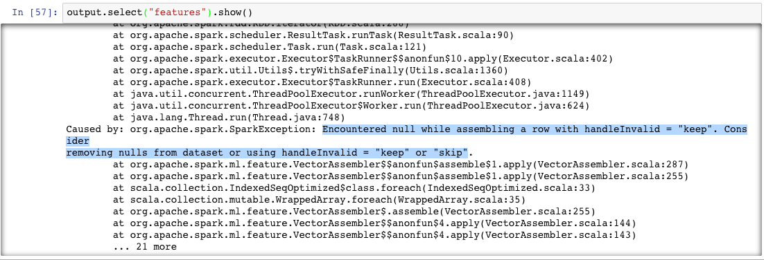
Error is pretty clear, while transforming data ML has encountered nulls in the data and is asking for a clarification of what needs to be done. We have two options, one, clean the data of null values and feed it back or tell ML packages to skip the null values. We will take the second route by adding an extra line in step 5
output = lassembler.setHandleInvalid("skip").transform(data)
Now, the code executes. Let’s see what’s there in the “features” output
output.select("features").show()
#output looks similar to below
+-----------------+
|         features|
+-----------------+
|  [4583.0,1508.0]|
|     [3000.0,0.0]|
|  [2583.0,2358.0]|
|     [6000.0,0.0]|
|  [5417.0,4196.0]|
|  [2333.0,1516.0]|
|  [3036.0,2504.0]|
|  [4006.0,1526.0]|
|[12841.0,10968.0]|
|   [3200.0,700.0]|
|  [2500.0,1840.0]|
|  [3073.0,8106.0]|
|  [1853.0,2840.0]|
|  [1299.0,1086.0]|
|     [4950.0,0.0]|
|     [3596.0,0.0]|
|     [3510.0,0.0]|
|     [4887.0,0.0]|
|  [2600.0,3500.0]|
|     [7660.0,0.0]|
+-----------------+
only showing top 20 rows
6. Let’s now feed this input Vector and our prediction value(Y), which is ‘LoanAmount’
loan_data = output.select('features','LoanAmount')
loan_data.show()
#and Output is
+-----------------+----------+
|         features|LoanAmount|
+-----------------+----------+
|  [4583.0,1508.0]|       128|
|     [3000.0,0.0]|        66|
|  [2583.0,2358.0]|       120|
|     [6000.0,0.0]|       141|
|  [5417.0,4196.0]|       267|
|  [2333.0,1516.0]|        95|
|  [3036.0,2504.0]|       158|
|  [4006.0,1526.0]|       168|
|[12841.0,10968.0]|       349|
|   [3200.0,700.0]|        70|
|  [2500.0,1840.0]|       109|
|  [3073.0,8106.0]|       200|
|  [1853.0,2840.0]|       114|
|  [1299.0,1086.0]|        17|
|     [4950.0,0.0]|       125|
|     [3596.0,0.0]|       100|
|     [3510.0,0.0]|        76|
|     [4887.0,0.0]|       133|
|  [2600.0,3500.0]|       115|
|     [7660.0,0.0]|       104|
+-----------------+----------+
only showing top 20 rows
7. Standard practice is to divide the test data into 2 parts- train the ML model with the first and let it predict the values on second set, so we can crosscheck the performance.
#splitting train and test data into 70% and 30% of total data available
train_data,test_data = loan_data.randomSplit([0.7,0.3])

#finally, calling the linear regression package we imported
lr = LinearRegression(labelCol='LoanAmount')
#we are specifying our 'Y' by explicitly mentioned it with 'labelCol'

#fitting the model to train data set
lrModel = lr.fit(train_data)
When you run the above, you should get an output like below
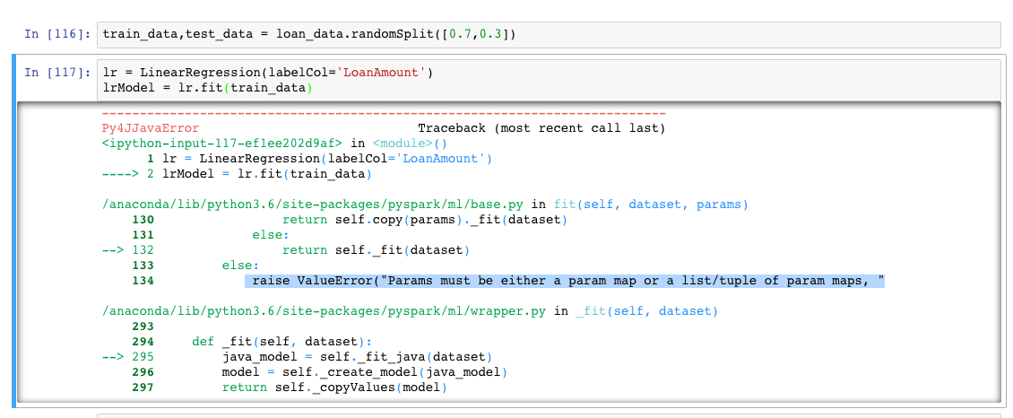
The error says – “Params must be either a param map…”. Reason for this error is our dependent variable (LoanAmount) has null values and ML cannot fit a model which as null as output values. There are lot of ways to clean this kind of data, we will not consider null values in our example. Let’s filter out null ‘LoanAmount’ values when we read the data from csv itself like so:
data = spark.read.csv("train.csv",inferSchema=True,header=True)
#we will add a filter to remove the null values from our dependent variable
data = data.filter("LoanAmount is not NULL")
data.printSchema()
Repeat the steps above and the error will go away. So, our Linear regression Model is ready now.
8. Let’s check the residuals (residual = observed value(the value in our input) – predicted value (value predicted by the model) of Y). Each data point will have one residual. So, number of residuals will be equal to the number of records we fed as input.
test_results = lrModel.evaluate(test_data)
test_results.residuals.show()
#output looks similar to below
+--------------------+
|           residuals|
+--------------------+
|5.684341886080801...|
|-1.42108547152020...|
|-4.26325641456060...|
|-1.42108547152020...|
|-1.42108547152020...|
|-2.84217094304040...|
|-1.42108547152020...|
|-1.42108547152020...|
|-1.42108547152020...|
|-1.42108547152020...|
|                 0.0|
|-1.42108547152020...|
|-2.13162820728030...|
|-1.42108547152020...|
|-2.84217094304040...|
|                 0.0|
|2.842170943040400...|
|-1.42108547152020...|
|-1.42108547152020...|
|-3.55271367880050...|
+--------------------+
only showing top 20 rows
9. Voila, we can now use this model to predict output of our test data
predictions_data = test_data.select('features')
predictions = lrModel.transform(predictions_data)
predictions.show()
Comments